Analyzing JMeter Results with R

"If you can't measure it, you can't manage it."
— Peter Drucker
To be able to improve a system's performance I need to understand the current characteristics of its operation. So I created a very simple (you might call it naïve as well) performance test with JMeter. Executing the test for roughly 35 minutes resulted in 386629 lines of raw CSV data. But raw data does not provide any insight. In order to understand what is going on I needed some statistical numbers and charts. This is where R comes into play. Reading data in is quite simple:

/response-times.R

responseTimes<-read.table("response-times.csv",header=TRUE,sep=",")

First of all, I wanted an overview of the latency over the test runtime.

/response-times.R

plot((responseTimes$timeStamp-min(responseTimes$timeStamp))/1000/60,
     responseTimes$Latency,
     xlab="Test time [min]",
     ylab="Latency [ms]",
     col="dodgerblue4",
     pch=18
)

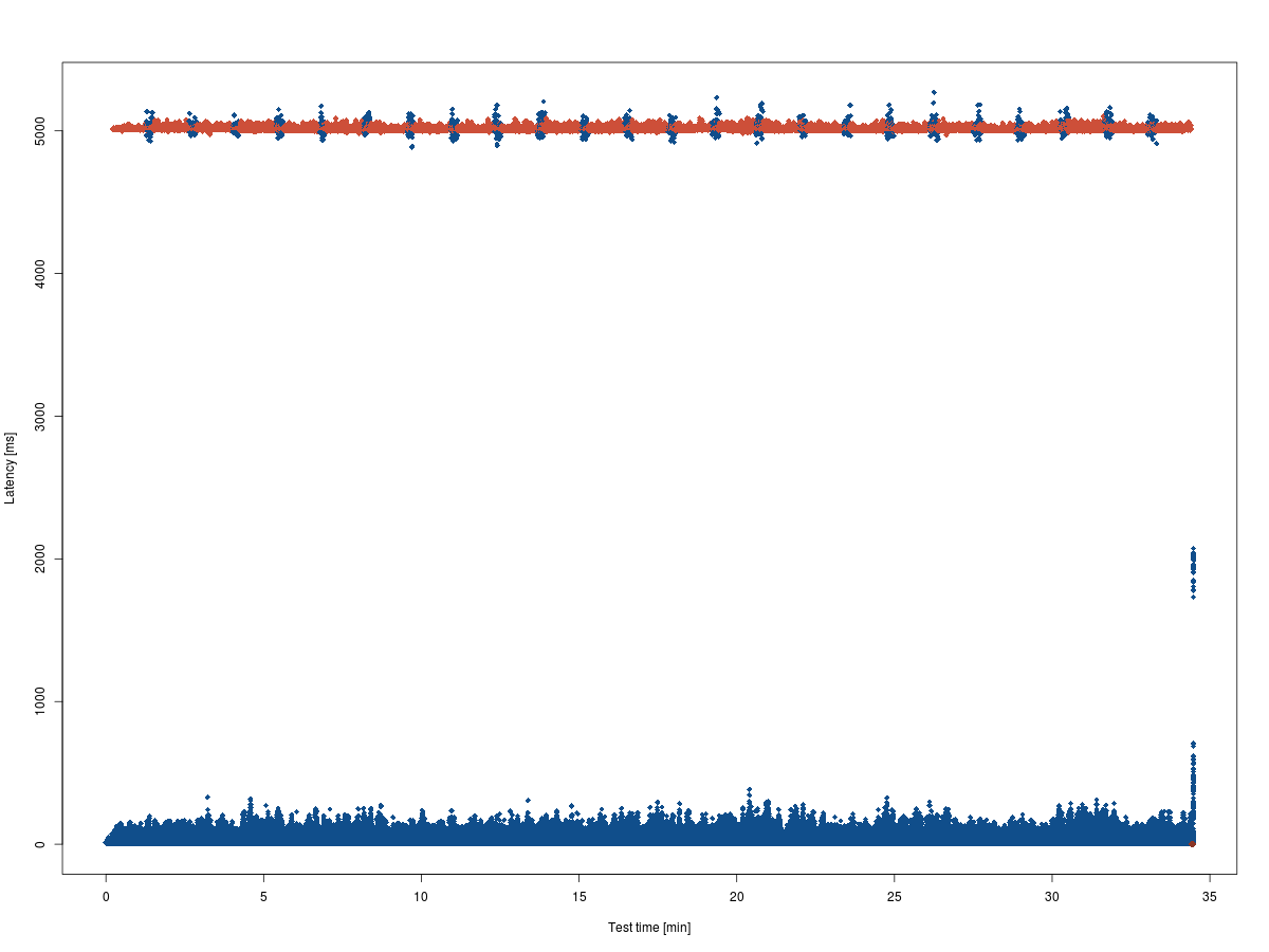
Response times seem to be pretty stable over time, I cannot identify any trends at first sight. Nevertheless, the results are split: requests are replied to either quite fast or after about 5 seconds. The "five second barrier" is interesting, though. It is too constant to be incidental. This begs for further investigation.
As a next step, I analyzed the ratios of HTTP response codes during the test:

/response-times.R

par(lwd=4)
pie(summary(responseTimes$responseCode),
    clockwise=TRUE,
    col=c("steelblue3", "tomato2", "tomato3"),
    border=c("steelblue4","tomato4","tomato4"),
    main="HTTP Response Codes"
)

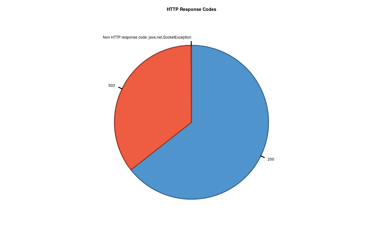
About 2/3 of the requests are handled successfully, but 1/3 of the requests resulted in server errors. That's definitely too many and needs improvements.
As a last, but very important step, I analyzed the overall service levels. So I created a plot of the cumulated relative frequency of the response times.

/response-times.R

plot(ecdf(responseTimes$Latency),
     main="Cumulative relative frequency of response times",
     xlab="Latency [ms]",
     ylab="Quantiles",
     pch=18
)

Important indicators are usability barriers and the 95 percentile. Regarding usability, the ultimate goal are 100 ms response time; this makes the system appear instantaneous. 1000 ms response time are the maximum not to interrupt the user's flow of thought.

/response-times.R

axis(1,at=c(100),labels=c("100"),col="green4")
instantResponse = cumsum(table(cut(responseTimes$Latency,c(0,100))))/nrow(responseTimes)
segments(100,-1,100,instantResponse,col="palegreen3",lty="dashed",lwd=2)
points(c(100),instantResponse,col="green4",pch=19)
text(100,instantResponse,paste(format(instantResponse*100,digits=3), "%"),col="green4",adj=c(1.1,-.3))

fastResponse = cumsum(table(cut(responseTimes$Latency,c(0,1000))))/nrow(responseTimes)
segments(1000,-1,1000,fastResponse,col="palegreen3",lty="dashed",lwd=2)
points(c(1000),fastResponse,col="green4",pch=19)
text(1000,fastResponse,paste(format(fastResponse*100,digits=3), "%"),col="green4",adj=c(1.1,-.3))

The 95 percentile is the "realistic maximum" response time. Beyond this limit are the extreme outliers that you cannot prevent on a loosely coupled, unreliable, distributed system like the internet. Fighting against these is a waste of your valuable time. But for service quality, it is important that nearly every user gets a reasonable response time. In order to calculate and plot the 95 percentile, I had to:

/response-times.R

axis(2,at=c(0,.1,.2,.3,.4,.5,.6,.7,.8,.9,.95,1),labels=FALSE)
axis(2,at=c(.95),labels=c("95%"),col="tomato3")
ninetyfiveQuantile = quantile(responseTimes$Latency,c(0.95))
segments(-10000, 0.95, ninetyfiveQuantile, .95, col="tomato1",lty="dashed",lwd=2)
points(ninetyfiveQuantile,c(0.95),col="red3",pch=19)
text(ninetyfiveQuantile,c(0.95),paste(format(ninetyfiveQuantile),"ms"),col="red3",adj=c(-.1,1.3))

These calculations result in the following plot.

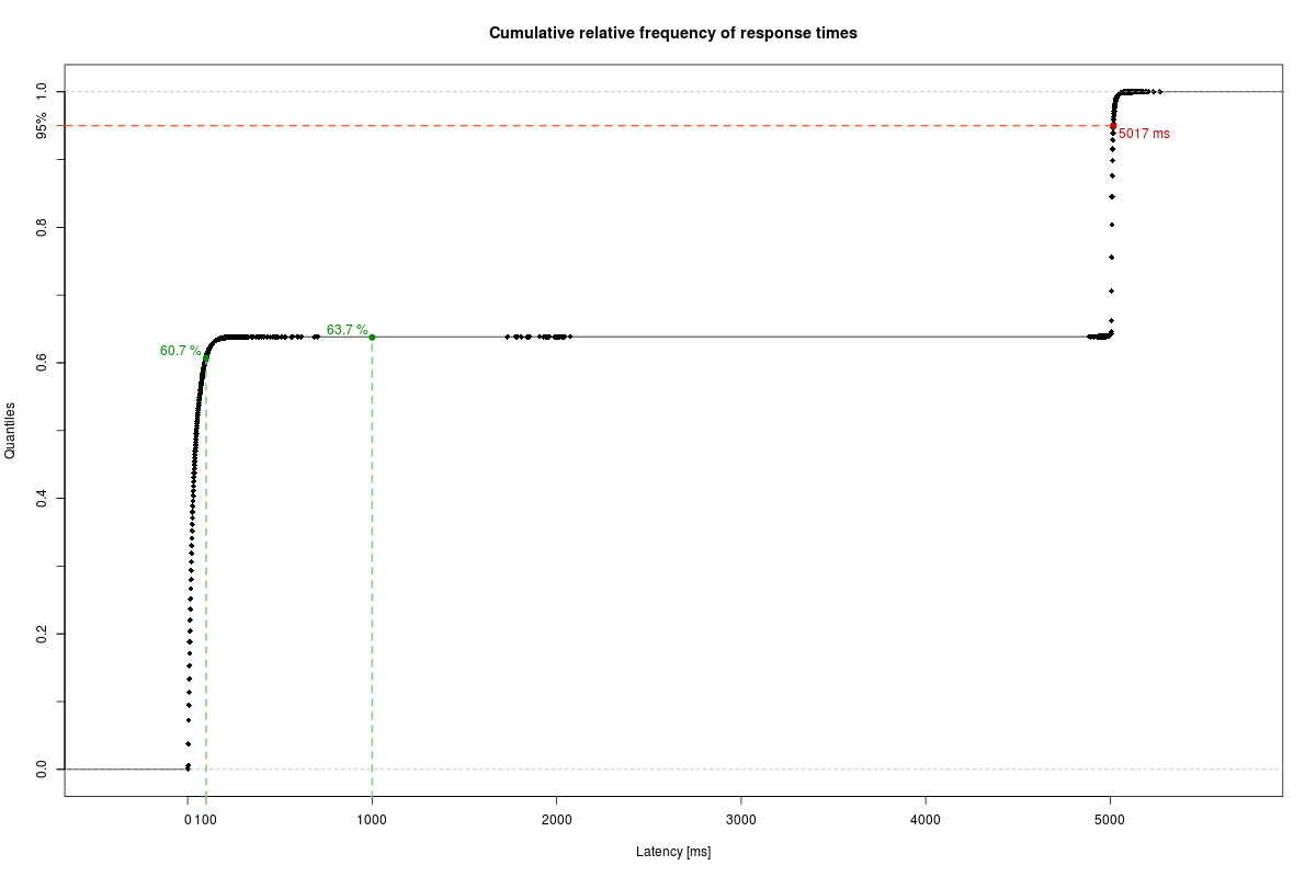
To sum it up, the system is able to

• serve 60.7 % of its users in 100 ms or less;
• serve 63.7 % of its users in 1000 ms or less;
• serve 95 % of its users in 5017 ms or less.

It seems very likely that the successful requests are responded quickly, and that the responses that took about 5 seconds are the 503 errors. The timeout is probably caused by some kind of bottleneck. I did not investigate this further yet, but I am quite happy with the visualizations I produced.
As always, the sources are available via GitHub.
References:

• Advanced graphs
• Intermediate plotting
• An Introduction to R
• Kickstarting R — Plotting data – point/line graphs
• R color names
• R data import/export
• The R Graphics cookbook